Imagine you’re in the middle of an important meeting, and your manager suddenly asks you for the total sales figures for specific months from your company’s Google Sheets. You know that calculating this manually would take too much time. That’s where the SUM formula comes to the rescue, allowing you to quickly sum up your data in seconds.
In this guide, you’ll discover just how easy it is to sum columns in Google Sheets, no matter the complexity of your data. By the end, you’ll be confidently managing your data and making quick work of any sum in a Google spreadsheet.
How to Sum the columns in 5 ways
You can sum up columns in Google Sheets in more ways than you might think. Also, each method has its own advantages. If you're after a quick fix or need something more specific, we've got you covered. These methods will help you to get quick and correct results, no matter how simple or complex your spreadsheet is.
1. AutoSum feature
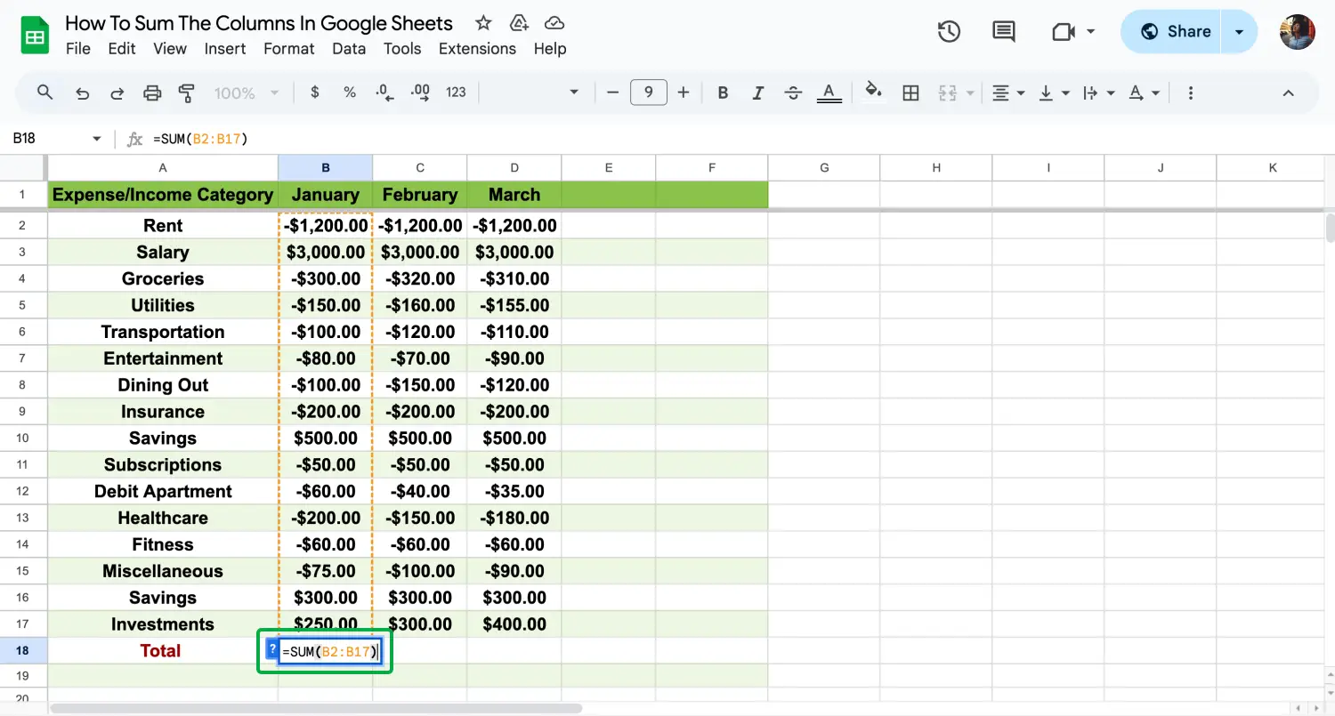
AutoSum feature of Google Sheets
The AutoSum feature lets you sum up a range of cells with just one click. Our finance sheet uses AutoSum in cell B18 to quickly calculate total January expenses. One simple step: we just type the = (equal) symbol in B18, and Google Sheets will instantly suggest the =SUM(B2:B17) formula. Press Enter to accept the suggestion, and we can display the desired result in seconds.
2. Using the SUM formula
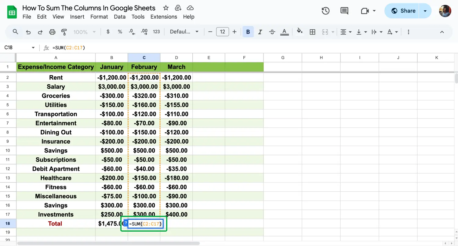
Use the SUM formula
The SUM formula adds values in a column by typing =SUM(range). For our example, we calculate the total February expenses by summing all items in cell C18 using =SUM(C2:C17). After you clarify the range and Enter the formula, whenever you choose the cell, Google Sheets draws colorful lines to preview your range.
3. SUMIF formula
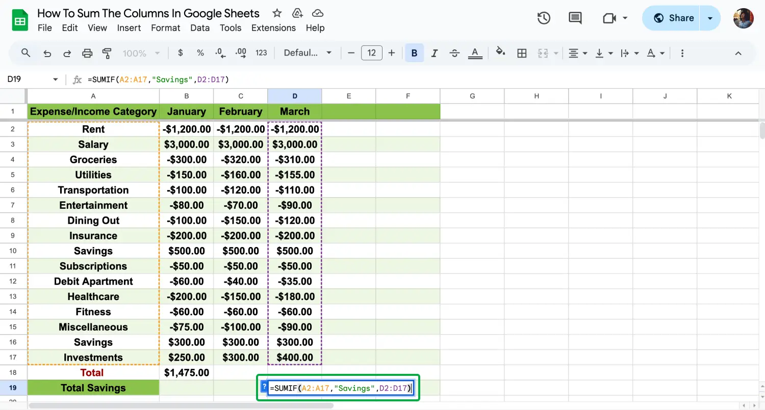
Use the SUMIF formula
The Google Sheets sum if the values meet specific criteria. In our example, we sum only the "Savings" category in March by using =SUMIF(A2:A17, "Savings”, D2:D17). This method is proper when you need to focus on specific categories or conditions, like filtering expenses by type.
4. Array formula
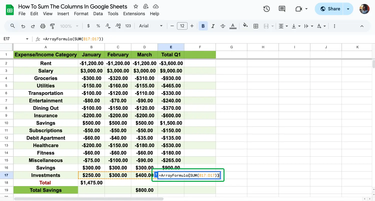
Use the Array formula
Array formula in Google Sheets sum multiple columns or rows at once. We use it to calculate Q1 total expenses for Rent with =ArrayFormula(SUM(B3:D3)), summing January through March. This is great for handling large datasets or when you must simultaneously sum multiple columns.
💡 If you drag your Google Sheets formulas from the bottom right corner, it will automatically copy the formula to all the lines below to save you time.
5. Using cell references in formulas
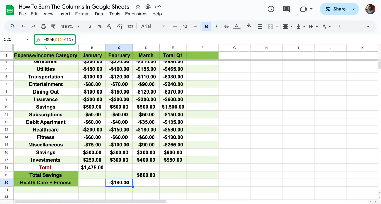
Use cell references in the formula
This method involves manually adding values from specific cells. In our example, we sum up the health and fitness expenses for the months. Firstly, we chose our cell to display the result and typed our formula =SUM(C12+B13) to calculate total Health and Fitness expenses in January. After you choose the cells you want to sum, just click Enter and get your result.
3 expert tips while summing the columns
A small mistake, like an incorrect range or an extra decimal point, can make some wrong calculations when summing columns in Google Sheets. In this section, we share expert tips to help you avoid these errors and confidently use formulas like SUMIF to sum multiple columns accurately. These tips will make your work easier and more reliable:
1. Double-check your cell ranges
One common mistake is including an extra cell or missing one when selecting a range. Always double-check that your cell ranges are accurate before pressing Enter.
2. Use SUMIF for conditional sums
When you need to sum specific data based on criteria, the SUMIF function is your best friend. We just showed an essential use, but it has much more potential for complicated data sets. This formula is useful in Google Sheets when you need to sum data based on specific conditions. However, a standard error is that the range and sum range do not match correctly.
3. Avoid mixing data types
Mixing text strings and numbers in the same column can create errors in your sum calculations. Combining different data types in a column can prevent formulas from working correctly and lead to inaccurate results. Keeping numerical data separate from text is essential to ensure accurate calculations.
Frequently asked questions about summing the columns
Summing columns in Google Sheets is usually easy, but sometimes you might have a few question marks about how things work. If you are looking for the proper function in Google Sheets or trying to figure out a logical operation, we are here to clarify things and help you sum up your data more quickly.
You can easily add up the products of columns in Google Sheets with a simple formula. This lets you quickly get the total you need without doing it all by hand. It’s an easy way to calculate your data fast.
Auto summing in Google Sheets is really easy. Just a couple of clicks and Google Sheets will add up your numbers automatically. You don’t have to type in the formula yourself, which saves time and makes your work quicker.
Making a running total in Google Sheets is simple and helps you keep track of your totals as you add more data. It updates by itself, so you can always see how much you’ve added up so far.
If you want to add up just certain cells in Google Sheets, you can do that easily by selecting the specific ones you need. Just type the formula starting =SUM( )and put the cells you want in parentheses. It’s useful when you don’t want to summarize the whole column, just a few parts.
Using SUMIF in Google Sheets is really simple. This function helps you add up numbers that meet a certain condition. Just choose the range you want to check, set your condition, and then select the cell, cells, or range to sum. It’s a handy way to get exactly the totals you need.
Key points to take away
Summing columns in Google Sheets is easier than you might think. With the tips and methods we've covered, you can quickly and accurately sum up your data. Remember to check your ranges and keep your data types consistent. If you want to know more about Google Sheets, just stay tuned for our guides. We are happy to help you to discover the potential of Google Sheets.
Behçet is a content writer at forms.app. He is a music producer and enjoys blending electronic and acoustic tunes. Behçet has expertise in Google Sheets, survey questions, and online forms.
